Table of Contents

My personal notes that helped me understand transformers. I’m a C programmer working at the systems and networking middleware level (RDMA, collectives). However, at NVIDIA it is becoming increasingly helpful to understand LLMs–even as a networking dev–because frontier models are giant enough that the entire cluster from the hardware up to the LLM itself all needs to be co-designed to get the best performance. Even a few % reduction in latency can save a lot of money in a large scale training run.

Introduction #

The modern AI era is huge. With investments as big as half a trillion (!) dollars coming from the Stargate Project, it’s hard to believe it would have been this big if the Vaswani et al paper Attention Is all You Need had not introduced the Transformer, which has become the dominant architecture for all types of models not limited to text generation.

Attention is at the heart of the transformer. With that, it was worth the effort to understand it enough that I could write a blog post on it and also the rest of the transformer. This is the culmination of that effort. The rest of this post is organized as follows: Attention in Context, The Complete Tensor Math of a Transformer, Multi-Head Attention (MHA), and Inference with KV-Caching which explains what Prefill and Decode are, and how KV-Caching can improve performance. Lastly, I end the post with a Conclusion and Acknowledgements.

Attention in Context #

In the Attention Is all You Need paper, they show this diagram:

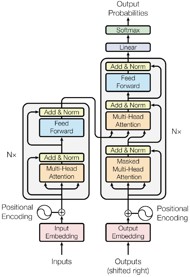
Figure 1: Transformer figure from the Attention is All You Need paper

This is the architecture of the original Transformer. You may have seen it before, especially since it has been reproduced so many times that one of the authors had to update the arxiv preprint to have big red text saying you’re allowed to do so at the top of the paper.

The left side is called the encoder–its job is to take the input tokens and produce a sequence of contextual representations. That sounds vague, but that’s because it is: the encoder by itself can be used for classification, sentiment analysis, search rankings, question answering, and so on. BERT is an example of an encoder-only model. However, the T5 model that came after this paper was used for Natural Language Processing (NLP) tasks, such as translating from one language to another (e.g, English to German). In this respect, the Encoder gathers the meaning of the entire text to be translated. Each token attends to–I will define the meaning of this shortly–every other token in the sequence. This is what self-attention is.

The decoder on the right side of the image takes the full output of the encoder, and builds the output autoregressively–that is, one token at a time by feeding the new token back in. The first attention layer in the decoder is causal-masked self attention. Causal-masking refers to setting attention scores of future tokens to $-\infty$, only allowing the model to make a prediction using the tokens seen so far. The second attention layer does cross attention, which has the token sequence attend to contextual sequence created by the encoder.

For autoregressive language modeling the encoder is actually not necessary, so the vast majority of models released these days are decoder-only models. This is due to several reasons:

Text is largely causal: That means it can be simpler and more effective to just predict the next token in the sequence instead of masking random tokens like you do with enc-dec or enc-only
Scale: The GPT-3 paper found that scale is extremely powerful and there are distinct widths of the attention and MLP blocks required to perform more challenging tasks, as well as distinct depths so that the model can write to the residual stream enough to handle tasks like reasoning. Therefore it’s often better to have a 10B decoder-only model than 5B in the encoder and 5B in the decoder
Design simplicity: It’s just easier to engineer a single unified model, since separating the encoder and decoder introduces load balancing, parallelism topology complexity, and additional synchronization points.

So, for the rest of this blog I will refer to their design instead of encoder-only or encoder-decoder models.

Note: Interestingly enough, Vaswani et al didn’t invent the attention mechanism, that was in https://arxiv.org/abs/1409.0473. Vaswani and team removed the recurrence from attention, added multihead attention (defined later), added an MLP, added positional encodings, and scaled it all up.

The Complete Tensor Math of a Transformer #

There are a lot of tools like this great visualizer, but for me, it didn’t click until I learned how to think in terms of shapes and operations abstractly like in this post. If you continue reading and still find it confusing: look up broadcasts, reductions, and pointwise operations and use numpy or pytorch to come up with a few examples.

For the rest of this post I’ll walk through a GPT-2 style model because it’s easy to digest, and because Karpathy’s minGPT provides a very nice educational implementation that you can try immediately after reading this blog.

Writing Convention #

@ means matrix multiplication. This is actually Python’s syntax. # is a comment also like in Python.

Here’s an example program illustrating two matrix multiplications and an activation function. It defines 3 tensors, the input $x$, and two weight matrices with their sizes shown in the comment.

I’ll define the tensors that are given by the user and the weights from the model file (e.g. the file you would download from Hugging Face) using $\in$:

$$ \begin{aligned} x &\in [M, K] \\ W_1 &\in [K, 4N] \\ W_2 &\in [4N, N] \\ \end{aligned} $$

Then in the program, I’ll use Python-like assignments:

x = x @ W_1 # [M, 4N]
x = GeLU(x) # [M, 4N]
x = x @ W_2 # [M, N]

The comments show the output shape of the operation. So, we multiplied $x$ by $W_1$, then GeLU’d it, then multiplied that by $W_2$. The final tensor’s shape is $[M, N]$.

Definitions #

Let

$B$ = “Batch size”, the number of independent token groupings we want to run through the model at a given time. If $B = 10$, you can think of it like 10 users chatting with Claude at a time. Or 10 different samples given to the model during training.

$S$ = “Sequence length”, the maximum length of all users’ chats in the batch. Say that each user wrote their own sentence, and the longest sentence among the users is 100 tokens. Then $S$ would be 100, and for the rest of the users whose sentence length is less than that the remaining tokens are filled with a padding that explicitly means “ignore this”. This is different from context length ($S_{\mathrm{max}}$), which is the maximum size of $S$ the model can handle.

$D$ = “Hidden size (or hidden dimension)”, the size of each token’s contextual representation. This a $D$-dimensional space, where each direction or combination of directions in the space has some meaning. You can think of it like this:

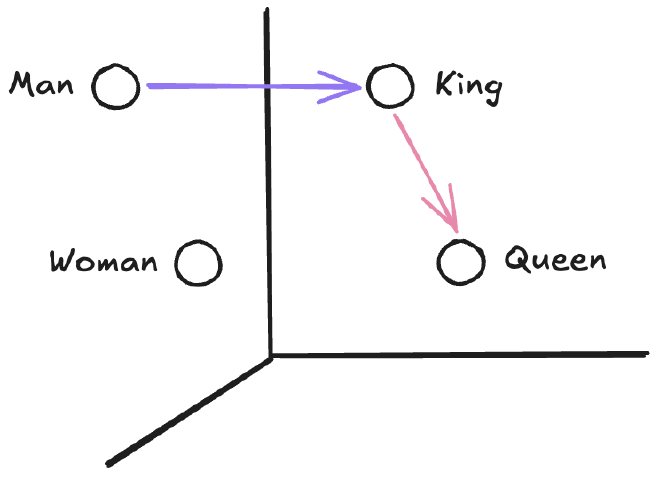
Here we have a direction for gender and a direction for royalty. The purple arrow shows the direction of royalty and the pink arrow shows the direction of femininity. You can start from any of the four points and add or subtract gender and royalty to get the others. What’s interesting is that all of the model’s knowledge is encoded in a space like this, even though it may not be as clean looking as this figure.

$V_{\mathrm{vocab}}$ = “Vocabulary size”, the number of different tokens there are.

$L$ = “Number of transformer layers” the model has, where each layer is one attention block & MLP block together.

Each of these are called hyper-parameters because they are configured by the model designer. GPT-2 small had $L = 12$, $V_{\mathrm{vocab}} = 50257$, $S_{\mathrm{max}} = 1024$, $D = 768$.

The Flow of Tokens #

Going bottom-up from Figure 1 and ignoring the encoder side (decoder-only), we have the following flow of tokens with my added illustrations.

Input to Embeddings #

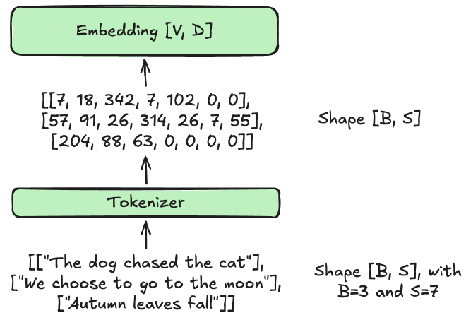
Figure 3: Input to tokens to start of embedding

The 3 users type their sentences, and the tokenizer (not pictured in Figure 1) converts the text string into an array of token IDs. This makes the input tensor to the model of shape $[B, S]$.

Each complete word may not actually correspond to a token ID, for example the word “unnecessary” might map to two tokens, un/necessary. This is the reason behind the old issue of counting the number of r’s in the word strawberry.

The next operation is an embedding table with a matrix $E \in [V_{\mathrm{vocab}}, D]$ that converts the tensor from shape $[B, S]$ to shape $[B, S, D]$. The purpose of the embedding is to expand each token ID into the vector in the $D$-dimensional space that represents that token’s meaning. This is NOT a matrix multiplication. The operation takes in a row number and returns that row from the embedding matrix.

Converting from shape [B, S] of token IDs to the [B, S, D] tensor of embeddings — Figure 4: Converting from shape $[B, S]$ of token IDs to the $[B, S, D]$ tensor of embeddings

Positional Embedding #

Now, we have a tensor of shape $[B, S, D]$. Next is the position embedding $P \in [S, D]$. The purpose is to encode the position of each token in the sequence. We broadcast add the position across every batch: $[B, S, D] + [S, D] = [B, S, D]$.

In GPT-2, the learned positional embedding table is $P_{\mathrm{table}} \in [S_{\mathrm{max}}, D]$. Each row corresponds to a position. So P_table[0, :] corresponds to position 0, P_table[1, :] position 1, …, then for getting $P$ we can take the slice: P = P_table[:S, :], i.e., skip everything after $S$.

Adding position to the token is helpful because the attention operation is a matrix multiply comparing every token to every other token without order, so to eventually capture that the dog is the one chasing in “the dog chased the cat”, we have to encode that the dog is first in the sentence inside of the dog token itself.

Transformer Layer #

Now, we enter the transformer layer itself. The first operation is LayerNorm, but that doesn’t change the shape so I won’t go into detail about it here. Just know it’s used to stabilize the training process. The transformer layer has two blocks–Attention and the Multi-Layer Perceptron (MLP). First is the attention block:

Attention Block #

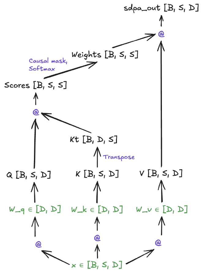
Figure 5: Scaled Dot-Product Attention shape transformations. Operations are purple, given tensors are green.

So, at the bottom we have the input $x \in [B, S, D]$.

Going upwards, you can see the attention block has three weight matrices, each of shape $[D, D]$

$$ \begin{aligned} W_q &\in [D, D] \\ W_k &\in [D, D] \\ W_v &\in [D, D] \\ \end{aligned} $$

Note: A lot of the time, $W_q$, $W_k$, and $W_v$ are concatenated into a single $W_{\mathrm{qkv}}$. The effect is the same though–there’s just one bigger multiply instead of three smaller multiplies.

We create three new tensors by multiplying with the weight matrices:

Q = x @ W_q # [B, S, D]
K = x @ W_k # [B, S, D]
V = x @ W_v # [B, S, D]

Run Scaled Dot Product Attention (here written without multihead attention, which is defined later):

Kt = K^T # [B, D, S]

scores = Q @ Kt # [B, S, S]
scores = scores / sqrt(D)

Apply the causal mask $m \in [S, S]$, whose upper right triangle is set to $-\infty$. Broadcast add. The shapes are unchanged:

scores = scores + m # [B, S, S]

Normalize the scores using softmax on the keys (the inner $S$ dimension):

weights = softmax(scores, dim=-1) # [B, S, S]

Now, each row sums to 1. The shapes are unchanged.

Note: You may have heard that attention is quadratic with respect to sequence length. Now you know why! Each batch has an $S$ by $S$ matrix.

Lastly, multiply by the $V$ matrix and the result is back to shape $[B, S, D]$ :

sdpa_out = weights @ V # [B, S, D]

Then, another linear is in the attention block (not pictured in Figure 5):

$$ \begin{aligned} W_o &\in [D, D] \\ \end{aligned} $$

attn_out = sdpa_out @ W_o # [B, S, D]

Dropout, Residual add, and another LayerNorm don’t change the shape.

Multi-Layer Perceptron (MLP) Block #

Then, each transformer layer has an MLP. It projects the hidden dimension up to $4D$, then back down to $D$, with an activation function in between:

$$ \begin{aligned} W1 &\in [D, 4D] \\ \end{aligned} $$

h = x @ W1 # [B, S, 4D]
h = GeLU(h)

$$ \begin{aligned} W2 &\in [4D, D] \\ \end{aligned} $$

mlp_out = h @ W2 # [B, S, D]

Lastly, there is another residual add, which doesn’t change the shape.

Getting the Output #

After passing through all $L$ transformer layers and a final LayerNorm, we get a new tensor $x$ with the familiar $[B, S, D]$ shape. Now, in order to get the next token prediction, we run a projection back to the vocabulary:

$$ \begin{aligned} W_{\mathrm{vocab}} &\in [D, V_{\mathrm{vocab}}] \\ \end{aligned} $$

logits = x @ W_vocab # [B, S, vocab_size]

Logits are the name for the raw scores of each potential token in the vocabulary. Using $V_{\mathrm{vocab}} = 50257$ means that each logits vector in the tensor has a certain score for all 50257 potential output tokens.

Note: When using embedding tying, $W_{\mathrm{vocab}}$ has the same weights as input embedding table: $W_{\mathrm{vocab}} = E^{\mathsf{T}}$. This is done to save on parameter budget.

During inference, we just take the last $S$: [:, S-1:S, :] (Python array slicing notation). This gives a $[B, 1, V_{\mathrm{vocab}}]$ tensor which has a single next-token prediction: a score (logit) for every token in the vocabulary. The final step is to softmax this tensor across the last dimension in order to convert the scores into a probability distribution that the model can sample from.

During training, however, all $S$ positions are used. Because of causal masking, the logits at each position predict the next token in the sequence without being influenced by future tokens. From there we can compute the loss for every index and run backpropagation to update the model’s weights.

Multi-Head Attention (MHA) #

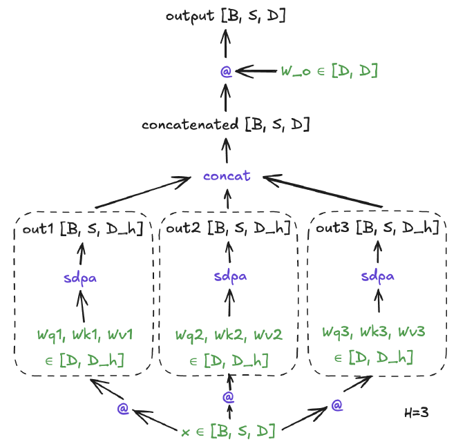
Figure 6: Multihead attention. Operations are purple, given tensors are green. Each head is its own box.

GPT-2 used MHA, but in the previous sections the shapes were made a little simpler by assuming we weren’t using it. At this point though, let’s add it back in. The steps to convert attention to MHA are to:

Split $D$ by the number of heads $H$ to get $D_h$, the dimension of each head. In GPT-2 small, $D_h=64$.
Then, for each head, train its own $W_{q,i}$, $W_{k,i}$, and $W_{v,i}$ matrices each of shape $[D, D_h]$, where $i$ is the ith attention head.
Do the SDPA calculation on each head–dividing the attention scores by $\sqrt{D_h}$ instead of $\sqrt{D}$–to get a tensor of size $[B, S, D_h]$.
Right before multiplying by the final $W_o$ projection, concatenate all head outputs back into the full $D$ sized tensor: $[B, S, D_h] \rightarrow [B, S, H\cdot D_h] = [B, S, D]$.

The idea is each head projects the same token into a smaller $D_h$-dimensional query/key/value space. The attention score between two tokens is then the dot product of their $D_h$-dimensional query and key vectors. Different heads have different learned projections, allowing them to learn different patterns. Figure 6 above illustrates the new flow.

Note: Going forward, we’ll disable MHA, so back to dividing by $\sqrt{D}$ instead of $\sqrt{D_h}$ after this section.

Inference with KV-Caching #

During inference there’s two stages: Prefill and Decode. Both stages without KV-caching are the same as what we’ve already covered. Since I found KV-caching to be really interesting, I wanted to share how it changes things here.

Prefill #

Say you start a new chat completely fresh. On the first time you hit enter to send your prompt to the model, it computes the attention scores normally, i.e., across the full sequence length $S$. That means every token gets compared to every other token. This is the same calculation as before:

$$ \begin{aligned} \text{Input } x &\in [B, S, D] \\ W_Q &\in [D, D] \\ W_K &\in [D, D] \\ W_V &\in [D, D] \\ \end{aligned} $$

Q = x @ W_q [B, S, D]
K = x @ W_k [B, S, D]
V = x @ W_v [B, S, D]

But with KV-caching enabled, store $K$ and $V$ for later, since they’ll be helpful in decode:

K_cached = K
V_cached = V

Finish running attention normally:

softmax((Q @ K.T) / sqrt(D) + m) @ V # [B, S, D]

Then continue on to the next transformer layer, with each one storing its own KV-cache like this one. The first token gets printed to screen by sampling the last $S$’s predicted probability distribution.

Decode #

Since the model is autoregressive, each new token gets added to the context and the whole process repeats with it. Without KV-caching, the decode stage is actually the same as the prefill stage, with each autoregression working with a sequence length one token longer than the last. However, the key insight behind KV-caching is that it makes decode only require computing a single new row in the attention matrices.

Here’s the flow. Instead of giving the whole sequence as an input, only the most recently generated token is given:

$$ \begin{aligned} \text{Input } x &\in [B, 1, D] \\ \end{aligned} $$

Q_new = x @ W_q [B, 1, D] # Notice these are single rows (S=1) per batch!
K_new = x @ W_k [B, 1, D]
V_new = x @ W_v [B, 1, D]

Append this token’s $K$ and $V$ row to the cache:

K_cached = K_cached.append(K_new) # [B, S+1, D]
V_cached = V_cached.append(V_new) # [B, S+1, D]

Run attention, but this time using K_cached and V_cached:

weights = softmax((Q_new @ K_cached.T) / sqrt(D)) # [B, 1, S+1]

The shapes for the above line are $[B, 1, D] \mathbin{@} [B, D, S+1] = [B, 1, S+1]$. The weights tensor holds the attention weights for just the input token over the previous tokens, instead of the S+1 tokens all against each other.

Multiply by V_cached to finish attention:

output = weights @ V_cached

The shapes of this are $[B, 1, S+1] \mathbin{@} [B, S+1, D] = [B, 1, D]$. We’ve converted it back to a single token. The net effect is that we’ve avoided recomputing $Q$, $K$, $V$, and attention outputs for all previous tokens. We compute $Q$, $K$, and $V$ only for the new token, append its $K$ and $V$ to the cache, and compute its query against all cached keys.

Conclusion #

To recap: the user’s input gets converted into token IDs, which get converted into a tensor of shape $[B, S, D]$. A transformer layer has an attention block which calculates $Q$, $K$, $V$ matrices, applies the famous $\operatorname{Attention} = \operatorname{softmax}\!\left(\frac{QK^{T}}{\sqrt{D}}\right)V$ equation, and then passes the result through an MLP. The process is repeated $L$ times before a final linear produces a $[B, S, V_{\mathrm{vocab}}]$ tensor over the vocabulary.

Inference has two modes, prefill and decode. Prefill processes the entire prompt in parallel, while decode computes attention one token at a time using stored $K$ and $V$ matrices.

Obviously transformers have evolved since GPT-2, so feel free to email me at nsarka00@gmail.com if you have any questions or comments. I’m happy to discuss these topics or even other topics related to networking and LLMs with you!

Acknowledgements #

Thanks to my longtime friends Quentin Anthony and Jacob Hatef for reviewing and making suggestions for this post.